Border Gateway Protocol (BGP) is not merely a protocol—it’s the backbone of the...


Request a personalized demo/review session of our Intelligent Routing Platform

Evaluate Noction IRP, and see how it meets your network optimization challenges

Schedule a one-on-one demonstration of our network traffic analysis product

Test drive NFA today with your own fully featured 30-day free trial

This eBook discusses the role of NetFlow as a valuable tool for collecting IP traffic matrices that can be used for capacity planning. The topic is separated into two main parts. The first part emphasizes the importance of network capacity planning and points out common pitfalls associated with this topic. It also provides an example of a NetFlow analysis practice in the process of investigation of network traffic that is not related to business and might be potentially harmful to your network. The second part focuses on the introduction to and the definition of internal and external traffic matrices, comparing their differences and usage. It also discusses the main methods for collecting and building traffic matrices based on NetFlow technology.
Network capacity planning is the process of planning a network for utilization, bandwidth, operations, availability in accordance with businesses needs. As the business evolves, a network needs to grow as well, in order to reflect increasing demands for network bandwidth. It is a common bias that it is sufficient to build the network with high-capacity devices and high-speed connections, so network infrastructure is ready to meet the future requirements for bandwidth.
This approach has several pitfalls associated with the cost. Firstly, it does not save investments as we might pay for something that we actually do not need, or it is an overkill. Bandwidth is not utilized and money is wasted for buying capacity that is not needed at all. On the other hand, user traffic on the network has a tendency to expand to fill the available bandwidth, whether or not it is crucial to the business. Also, in this case, the available bandwidth is not used effectively.
Secondly, even if the design may meet legitimate business-bandwidth requirements so it is within expected parameters for 90%, inappropriate network traffic such as DDoS, excessive downloading or file sharing can significantly exceed the capacity of the network. This might have a negative impact on legitimate traffic, degrading network performance and availability. For example, your customers may experience different types of issues, such as propagation delays, network outages that slow down or prevent access to provided services. As a result, the business may suffer significant financial losses. In the worst case scenario, the biggest and most important asset – the company’s reputation might be put in danger.
NetFlow provides a great insight into traffic that is flowing within, in or out of your network. NetFlow does not only offer historical reports about network utilization and performance but it can provide more detailed information about traffic. This is very important and helpful in the process of investigation of problems that cause congestion. For instance, why the number of SSH flows and packets measured by NetFlow is the highest in a network traffic graph depicted in Picture 1, while as for the average bit rate per second (bps), SSH is only on the third place? This might refer to SSH force attack that is well known for generating many small flows in terms of packet per flows (ppf) and bytes per flows (bpf). This kind of traffic, however, is not something that occurs regularly. Instead of buying additional bandwidth, one should take precautions that eliminate brute force attacks. For example, changing an SSH port or allowing access to the port for management IP addresses might significantly reduce of brute-force attempts.
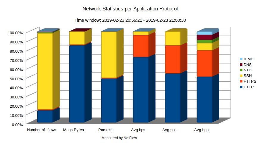
Figure 1: Network Statistics per Application Protocol.
[wc_divider style=”solid” line=”single” margin_top=”” margin_bottom=””]
The next logical step for network administrators would be finding out the IP addresses of the hosts that are targets of SSH brute force attack. This is where NetFlow comes in handy, again. For instance, the chart shown in Picture 2 reveals that the host with the highest number of flows is 195.165.10.100. Most likely, it is the victim of SSH brute force attack.
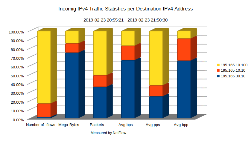
Figure 2: Incoming IPv4 Traffic Statistics per Destination IPv4 Address.
[wc_divider style=”solid” line=”single” margin_top=”” margin_bottom=””]
Filtering NetFlow records for IPv4 addresses matching our hosts and protocol SSH confirms that the victim of SSH brute force attack is the host 195.165.10.100 (Picture 3).
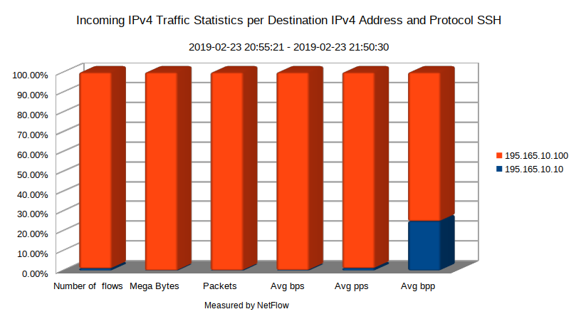
Figure 3: Incoming IPv4 Traffic Statistics per Destination IPv4 Address and Protocol SSH.
[wc_divider style=”solid” line=”single” margin_top=”” margin_bottom=””]
In order to eliminate the brute force attack against SSH protocol using firewall rules, we need to know the attacker’s IPv4 address. It can be easily done by filtering NetFlow records for source IP addresses. The source IP address with the highest number of flows is 10.10.10.10 (Picture 4). This IP address belongs to the private IP address range (RFC1918), so most likely the attack is launched from the inside network.
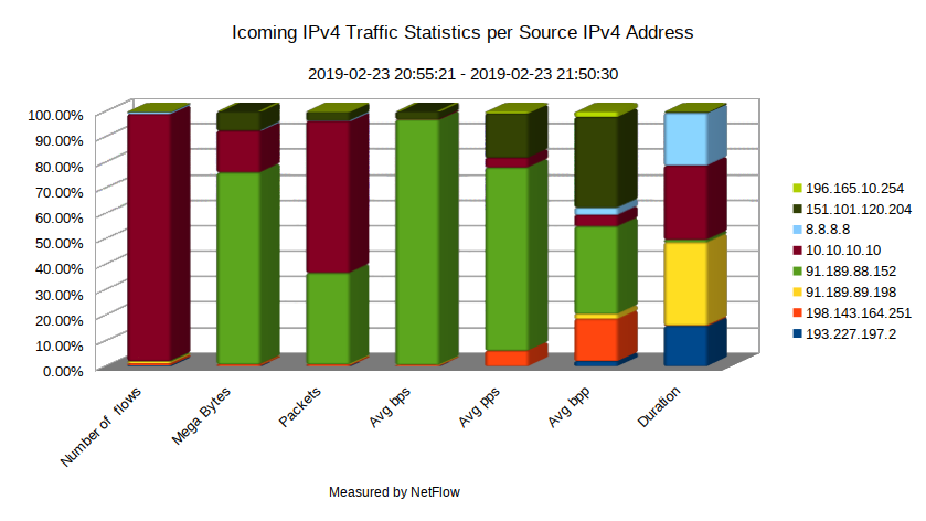
Figure 4: Incoming IPv4 Traffic Statistics per Source IP Address.
[wc_divider style=”solid” line=”single” margin_top=”” margin_bottom=””]
NetFlow can provide network statistics over a very short period of time, based on the configured active and inactive timeouts. If there is a suspicion that a link experiences congestion, it is necessary to collect NetFlow statistics about bandwidth utilization over a significant period of time. NetFlow collector must be able to provide a long-term view of utilization but sudden spikes of high utilization might be easily averaged out by this view. As a result, they will be hidden for network capacity planners. For this reason, the collector should provide insight into peak utilization, for instance showing the busiest minute or hour in a day. Based on the identified application protocols in NetFlow records, legitimate network traffic may be distinguished from non-business network traffic. Obviously, before spending funds on buying additional network capacity, we need to be sure that congestion and degraded application performance is caused by legitimate traffic. It helps to lower operational cost while keeping optimal network performance. This task can be hardly achieved without using the automated monitoring and reporting tool based on NetFlow.
A traffic matrix is a two-dimensional matrix with its ij-th element, tij determining the amount of traffic sourcing from node i and exiting at node j. The value tij is also called the traffic demand and each demand represents the amount of data transmitted between every pair of network nodes. In a network consisting of four nodes, where each node is a traffic source or a sink, traffic matrix contains 12 demands (Picture 5a). However, there are only four demands, when nodes 1 and 2 represent traffic sources and nodes 3, 4 are traffic destinations (Picture 5b).
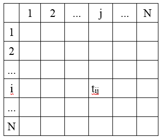
Table 1: Example of a Traffic Matrix.
[wc_divider style=”solid” line=”single” margin_top=”” margin_bottom=””]
| Note: The example of the traffic demand is 1.5Gbps from aen1.az.datacenter1.noction.com to bfm2.oh.noction.com. This traffic enters the network at aen1.az.datacenter1.noction.com and traverses the network along a certain path until it reaches bfm2.oh.noction.com, where it leaves the network on its way to an external AS. |
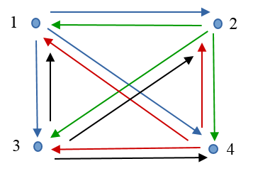
5a: Each Node is Traffic Source or Sink
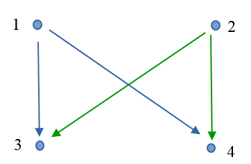
5b: Nodes 1, 2 are Traffic Sources and Nodes 3, 4 are Sinks
Figure 5: Number of Demands Related to Various Traffic Sources and Destinations.
[wc_divider style=”solid” line=”single” margin_top=”” margin_bottom=””]
Nodes 1, 2, …., N in Table 1 are the nodes located in the provider’s network. Each entry node can be an individual router, a specific interface of a router, a source prefix or a site that contains multiple routers – Point of Presence (PoP) (Picture 6). The exit node can be an individual router, PoP, a BGP next hop or MPLS Forwarding Equivalent Class (FEC), or a destination prefix. It is important to select a node in terms of the network size. For a large ISP, network PoP might represent a good choice because the size of the PoP traffic matrix is lower than the size of the router-level matrix. The amount of processed data and exported traffic to a collector is lower as well. On the other side, the granularity of the router-level matrix is higher (better) than the granularity of PoP-level matrix at the cost of generating more network traffic.
| Note: Most ISP networks are organized as a collection of points of presence (POPs) that form an ISP network. A POP is typically a collection of geographically co-located (or closely located) network nodes. Each POP is interconnected with one or more other POPs. Bandwidth between devices within a POP is relatively inexpensive compared to inter-POP connections, typically because the service provider owns the facility and can therefore easily interconnect nodes residing within the POP [1]. |
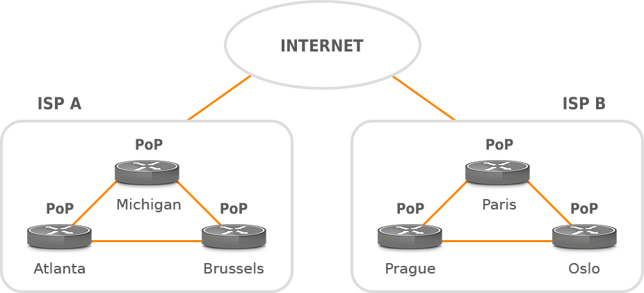
Figure 6: ISP PoP Network.
[wc_divider style=”solid” line=”single” margin_top=”” margin_bottom=””]
Basically, there are at least three good reasons for collecting and building a traffic matrix.
The traffic matrix depicts how much traffic enters the site, its distribution inside the site, and at what places the traffic exits the site. This information is very important for accurate network planning. For instance, let’s have a look at the network depicted in Picture 7. Traffic enters the network via routers R1 and R3 from an external network and leaves the site via routers R4 and R5. In case the traffic entering a network via router R1 increases, we cannot determine whether it adds load to the link between R2 and R4 or to the link between R2 and R5. Therefore, we need a traffic matrix to determine how the load will change on these two links so we can plan the link capacity accordingly.
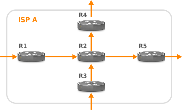
Figure 7: Example of Traffic Flows Within ISP A Network.
[wc_divider style=”solid” line=”single” margin_top=”” margin_bottom=””]
A traffic matrix can be used for resilience analysis of network under a failure condition. In case of the router R5 outage, the network topology is changed. All traffic is routed via R4 to an external network. With knowledge of a traffic matrix, ISP can successfully predict, whether there is sufficient free capacity on the link between R2 and R4 in order to sustain higher traffic demands.
The goal of optimization is to improve the performance of an ISP network. This includes finding bottlenecks and routing changes, so bandwidth can be utilized more effectively, reducing the time that traffic spent in an ISP network. For instance, if there are more BGP exit points in a network, traffic with higher priority should take the more optimal path to the nearest BGP router, while best-effort traffic can be sent to BGP peer via a suboptimal path. This cannot be accomplished without the knowledge of traffic matrix that provides information about the volume of traffic entering a network, where traffic leaves the network and how it is distributed within the ISP’s network.
Internal traffic matrix provides a look at traffic from the point of network core (between core routers) or between provider edge (PE) routers. Therefore, internal matrices are used for determining the impact of changes that occur within the network core. In order to reduce the size of an internal matrix in case of a large network, PoP-level matrix can be used instead of router-level. Picture 8 depicts traffic from two core routers to other core routers.
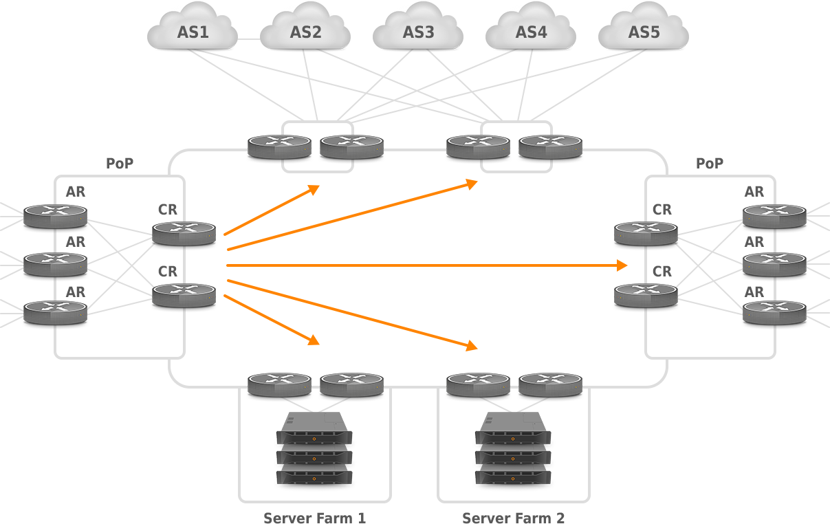
Figure 8: PoP to PoP Traffic for Internal Matrix.
(source: https://www.nanog.org/meetings/nanog34/presentations/telkamp.pdf)
[wc_divider style=”solid” line=”single” margin_top=”” margin_bottom=””]
External traffic matrix also provides information on where the traffic comes from entering a network and where it goes when exiting the network. The external core traffic matrix requires the previous/next BGP AS in the path, or the source/destination BGP AS, or the source/destination IP address or prefix. External matrix is useful for analyzing the impact of external failures on the core network (capacity/resilience), for example, when we lose a BGP peer so traffic is shifted between various Border Gateway Protocol (BGP) peering locations. Picture 9 depicts traffic that is exchanged between core routers on the left side and next-hop ASs.
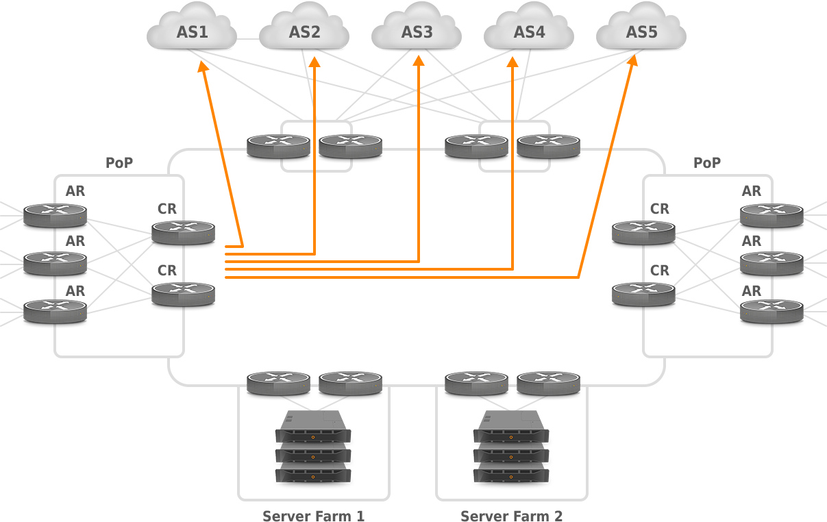
Figure 9: PoP to PoP with PE (AR) or CR for External Matrix.
(source: https://www.nanog.org/meetings/nanog34/presentations/telkamp.pdf)
[wc_divider style=”solid” line=”single” margin_top=”” margin_bottom=””]
Temporal distribution tells us how traffic is distributed over time. Picture 10 depicts aggregated traffic during a 24-hour time interval, with a minimum close to 6:00 hour and busy period that extends three hours. It is important to collect traffic matrix within the peak window in order to get accurate traffic rates needed for capacity planning and failure analysis.
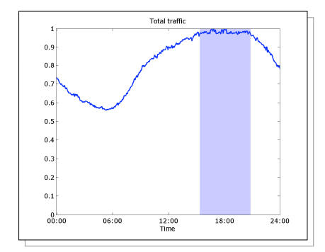
Figure 10: Total 24-hour Traffic Distribution Graph.
(source: https://www.nanog.org/meetings/nanog34/presentations/telkamp.pdf)
[wc_divider style=”solid” line=”single” margin_top=”” margin_bottom=””]
Spatial distribution provides information on how traffic gets distributed inside a network, whether traffic is evenly distributed or concentrated between a few sites (Picture 11). The source nodes are put on y-axis and the destination nodes are located on x-axis. The color indicates how much traffic passes between a pair of nodes, blue colors indicating minimum traffic and yellow/red color indicating a lot of traffic. Obviously, most of the traffic is distributed between a few nodes, so few large nodes contribute to the total traffic (20% demands – 80% of total traffic). These might be nodes with high customer concentration and BGP peering. The rule 80/20 is known as Pareto principle. It states that for many events, roughly 80% of the effects come from 20% of the causes.
| Note: Sometimes, it is useful to know how much traffic is distributed to other nodes so we need to calculate the fanout factor. Fanout factor is the relative amount of traffic (as a percentage of total) that nodes send to other sites. The higher a fanout factor, the more traffic is distributed to other sites. According to traffic measurement from Tier-1 IP backbone, fanout factors has been proven to be much more stable for the network than demands themselves [2]. |
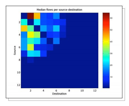
Figure 11: Spatial Traffic Distribution Graph.
(source: https://www.nanog.org/meetings/nanog34/presentations/telkamp.pdf)
[wc_divider style=”solid” line=”single” margin_top=”” margin_bottom=””]
Traffic matrix can represent peak traffic, or 95th percentile traffic, or traffic at a specific time. We use an appropriate traffic matrix depending on whether the network is provisioned based on peak traffic or 95th percentile traffic. The peak hour matrix for a large network with a lot of aggregate traffic is usually a good choice, as the sampling interval of 5 or 15 minutes is represented in the peak hour. Peak matrix is generated based on the collecting traffic for a certain time, e.g. day and peaks are calculated for a certain time period.
Matrices can be collected either in pull or push mode, depending on the preferred collection method. For instance, SNMP retrieves data from nodes in a pull mode, requesting bytes counters at fixed intervals, e.g, 5 or 15 minutes, depending on the required granularity level. However, byte counter values must be converted to rates. This can be achieved by collecting the values at multiple time intervals so the rate can be calculated based on the measured values and time.
NetFlow is a collection method that works in a push mode. When it is enabled on a router, it creates flow records based on the following criteria:
Each packet is examined for the above attributes. The first unique packet creates a flow as an entry in router’s NetFlow cache. The packet is then forwarded out of the interface. Other packets matching the same parameters are aggregated to the flow and the bytes counter for the flow increases. If any of the parameters is not matched, a new flow is created in the cache.
Flows are exported by a node to a collector when either inactive or active timeout expires or NetFlow cache is full. In that case, flows are exported using UDP or SCTP transport protocols, with UDP being more preferable, due to its speed and simplicity.
NetFlow must be enabled on the nodes where packets enter or exit network. Those are the CE facing interfaces of PE (AR) routers. The static method of converting NetFlow data to traffic matrix relies on the source and destination IP addresses within NetFlow records and a list of addresses generated for each customer. The IP addresses in a NetFlow record match the source and destination IP addresses of the packets. Having a generated list of IP addresses for each customer, we can determine a node where a packet exits the network. Therefore, we can create a traffic matrix that contains the source and destination node and traffic rate measured by NetFlow. The static method is not scalable thus applicable for large networks. The more convenient method is using communities or BGP AS exported in NetFlow records so BGP AS number can be used to find a node where traffic exits an ISP network.
NetFlow Version 8 adds router-based aggregation schemes that enable a router to summarize NetFlow data. This allows creating traffic matrices inside of a router so the amount of exported NetFlow data is reduced. As a result, bandwidth is not consumed by the export of NetFlow information that is not needed. When a flow expires, it is added to the aggregation cache of the router, instead of sending it to a collector. Flows are collected based on aggregation criteria. After 5 or 15 minutes, the aggregated flow is sent to a collector. Several aggregations schemes can be enabled at the same time such as Protocol port, AS, Source/Destination Prefix. For instance, the NetFlow AS Aggregation scheme groups data flows that have the same source BGP AS, destination BGP AS, input interface, and output interface. The aggregated NetFlow data export records report the following:
The BGP next hop presents the network’s exit point. Therefore, if we aggregate flows based on the BGP next hop TOS aggregation criterion, we can find on which peering router traffic leaves the network. The BGP NextHop TOS Aggregation scheme groups data flows that have the same BGP next hop, source BGP AS, destination BGP AS, input interface, and output interface. The aggregated NetFlow data export records report the following:
The NetFlow BGP Next Hop Aggregation provides an almost direct measurement of the traffic matrix. The drawback with this method is that only the prefixes in the BGP table are monitored. The routes that are not in the BGP table are reported with 0.0.0.0 as the BGP next hop.
A NetFlow collector machine with BGP daemon listening for BGP updates from ISP routers is known as the BGP passive peer on the NetFlow collector. The BGP daemon does not send any routes to other peers. When a collector receives flow records from exporters, it looks up the source and destination IP addresses in the BGP routing table and retrieves the AS numbers of ingress and egress routers. However, a BGP passive peer on the collector can return all the BGP attributes such as source and destination AS, second AS, AS Path, BGP communities, BGP next hop, etc. that can be used for creating traffic matrix.
The main advantage of this method is that an exporter doesn’t do CPU intensive look up in a BGP table. The amount of exported NetFlow data is also reduced as BGP related information are not added to flow records. This enables NetFlow version 5 to be used for flow export, although it does not support aggregation scheme based on BGP AS.
[wc_divider style=”solid” line=”single” margin_top=”” margin_bottom=””]
Network capacity planning ensures that enough capacity is always available despite the ever-increasing or often varying requirements. It is continuous and probably never ending process that helps to act proactively and avoid network performance degradation. A traffic matrix plays an important role in this process as it offers a clear picture of how much traffic enters the network, where, its distribution inside the network, and at what places the traffic exits the network. As we have discussed, NetFlow can be successfully used to collect traffic matrix in the provider’s BGP network. The performance of such a solution can be increased with the use of a BGP daemon on NetFlow collector. In this case, BGP related information can be gathered directly from the BGP table of a collector and associated with flow records.